Hogyan lehet automatikusan kitölteni, amikor beírja az Excel legördülő listát?

A sok elemet tartalmazó adatellenőrzési legördülő listához fel és le kell görgetnie a listában, hogy megtalálja a kívántat, vagy helyesen be kell írnia a teljes szót a listamezőbe. Van valami mód arra, hogy a legördülő lista automatikusan kitöltésre kerüljön a megfelelő karakterek beírásakor? Ezzel az emberek hatékonyabban dolgozhatnak a cellákban legördülő listákkal rendelkező munkalapokon. Ez az oktatóanyag két módszert kínál ennek elérésére.

A legördülő listák automatikus kiegészítése VBA-kóddal
Könnyen, 2 másodperc alatt automatikusan kiegészítheti a legördülő listákat
További útmutatók a legördülő listához ...

A legördülő listák automatikus kiegészítése VBA-kóddal

Kérjük, tegye a következőket, hogy a legördülő lista automatikusan kiegészüljön, miután beírta a megfelelő betűket a cellába.

Először be kell illesztenie egy kombinációs mezőt a munkalapba, és meg kell változtatnia annak tulajdonságait.

1. Nyissa meg azt a munkalapot, amely a legördülő lista celláit tartalmazza, amelyeket automatikusan kiegészíteni szeretne.
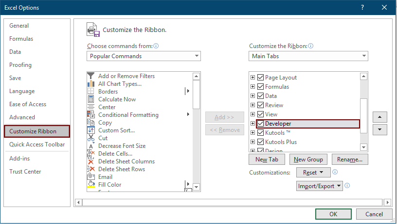
2. Kombinált mező beszúrása előtt hozzá kell adnia a Fejlesztő lapot az Excel szalaghoz. Ha a Fejlesztő lap látható a szalagon, váltás a 3. lépésre. Ellenkező esetben tegye a következőket, hogy a Fejlesztő lap megjelenjen a szalagon: Kattintson a gombra filé > Opciók megnyitni Opciók ablak. Ebben Excel beállítások ablakban kattintson Szalag szabása a bal oldali ablaktáblában ellenőrizze a Fejlesztő jelölőnégyzetet, majd kattintson a gombra OK gomb. Lásd a képernyőképet:
   
3. Kattints Fejlesztő > betétlap > Combo Box (ActiveX vezérlő).
   
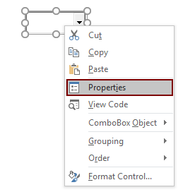
4. Rajzoljon egy kombinált mezőt az aktuális munkalapon. Kattintson rá jobb gombbal, majd válassza ki Ingatlanok a jobb egérgombbal kattintva.
   
5. A Ingatlanok párbeszédpanelt, kérjük, cserélje ki az eredeti szöveget a (Név) mezővel TempCombo.
   
6. Kapcsolja ki a Tervezési mód kattintson a gombra Fejlesztő > Tervezési mód.

Ezután alkalmazza az alábbi VBA kódot

1. Kattintson a jobb gombbal az aktuális lapfülre, majd kattintson a gombra Kód megtekintése a helyi menüből. Lásd a képernyőképet:
   
2. A megnyitón Microsoft Visual Basic for Applications ablakba, kérjük, másolja és illessze be az alábbi VBA kódot a munkalap Kód ablakába.
   VBA kód: Automatikus kitöltés, amikor a legördülő listába gépel

   Private Sub Worksheet_SelectionChange(ByVal Target As Range)
   'Update by Extendoffice: 2020/01/16
       Dim xCombox As OLEObject
       Dim xStr As String
       Dim xWs As Worksheet
       Dim xArr
       
       Set xWs = Application.ActiveSheet
       On Error Resume Next
       Set xCombox = xWs.OLEObjects("TempCombo")
       With xCombox
           .ListFillRange = ""
           .LinkedCell = ""
           .Visible = False
       End With
       If Target.Validation.Type = 3 Then
           Target.Validation.InCellDropdown = False
           Cancel = True
           xStr = Target.Validation.Formula1
           xStr = Right(xStr, Len(xStr) - 1)
           If xStr = "" Then Exit Sub
           With xCombox
               .Visible = True
               .Left = Target.Left
               .Top = Target.Top
               .Width = Target.Width + 5
               .Height = Target.Height + 5
               .ListFillRange = xStr
               If .ListFillRange = "" Then
                   xArr = Split(xStr, ",")
                   Me.TempCombo.List = xArr
               End If
               .LinkedCell = Target.Address
           End With
           xCombox.Activate
           Me.TempCombo.DropDown
       End If
   End Sub
   Private Sub TempCombo_KeyDown(ByVal KeyCode As MSForms.ReturnInteger, ByVal Shift As Integer)
       Select Case KeyCode
           Case 9
               Application.ActiveCell.Offset(0, 1).Activate
           Case 13
               Application.ActiveCell.Offset(1, 0).Activate
       End Select
   End Sub

   
3. nyomja meg más + Q gombok egyszerre a Microsoft Visual Basic alkalmazások ablak.

Mostantól, amikor egy legördülő lista cellára kattint, a legördülő lista automatikusan felszólítja. Elkezdheti beírni a betűt, hogy a megfelelő elem automatikusan teljes legyen a kiválasztott cellában. Lásd a képernyőképet:

Könnyen, 2 másodperc alatt automatikusan kiegészítheti a legördülő listát

A legtöbb Excel-felhasználó számára a fenti VBA-módszert nehéz elsajátítani. De a Kereshető legördülő lista jellemzője Kutools az Excel számára, egyszerűen engedélyezheti az automatikus kiegészítést az adatérvényesítési legördülő listákhoz egy meghatározott tartomány mindössze 2 másodperc alatt. Sőt, ez a funkció minden Excel-verzióhoz elérhető.

típus: Az eszköz alkalmazása előtt telepítse Kutools az Excel számára először. Menjen az ingyenes letöltéshez most.

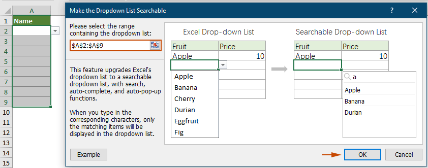
1. Ha engedélyezni szeretné az automatikus kiegészítést a legördülő listákban, először válassza ki a tartományt a legördülő listákkal. Ezután navigáljon a Kutools lapot választani Legördülő lista > A legördülő lista kereshetővé tétele, automatikusan előugró.
2. A Tegye kereshetővé a legördülő listát párbeszédpanelen kattintson a OK gombot a beállítás mentéséhez.

Eredmény

A konfiguráció befejezése után a megadott tartományon belüli legördülő lista cellájára kattintva megjelenik egy listamező. Karakterek beírásakor mindaddig, amíg egy elem pontosan egyezik, a teljes szó azonnal kiemelésre kerül a listamezőben, és egyszerűen az Enter billentyű megnyomásával feltölthető a legördülő lista cellájába.

Kapcsolódó cikkek:

A legjobb irodai hatékonyságnövelő eszközök

🤖	Kutools AI Aide: Forradalmasítsa az adatelemzést a következők alapján: Intelligens végrehajtás   |  Kód létrehozása  |  Hozzon létre egyéni képleteket  |  Adatok elemzése és diagramok létrehozása  |  A Kutools funkciók meghívása...
	Népszerű szolgáltatások: Ismétlődések keresése, kiemelése vagy azonosítása   |  Üres sorok törlése   |  Oszlopok vagy cellák kombinálása adatvesztés nélkül   |   Kerek Formula nélkül ...
	Szuper keresés: Több kritérium VLookup  |   Többértékű VLookup  |   VLookup több munkalapon   |   Fuzzy Lookup ....
	Speciális legördülő lista: Gyors legördülő lista létrehozása   |  Függő legördülő lista   |  Többszörösen válassza ki a legördülő listát ....
	Oszlopkezelő: Adjon meg egy adott számú oszlopot  |  Oszlopok mozgatása  |  Kapcsolja be a Rejtett oszlopok láthatósági állapotát  |  Tartományok és oszlopok összehasonlítása ...
	Kiemelt funkciók: Rács fókusz   |  Design nézet   |   Nagy Formula bár   |  Munkafüzet és lapkezelő   |  Erőforrás-könyvtár (Auto szöveg)   |  Dátumválasztó   |  Kombinálja a munkalapokat   |  Cellák titkosítása/dekódolása   |  E-mailek küldése listánként   |  Szuper szűrő   |   Speciális szűrő (félkövér/dőlt/áthúzott szűrés...) ...
	A 15 legjobb eszközkészlet:  12 szöveg Eszközök (Szöveg hozzáadása, Karakterek eltávolítása,...)   |   50 + Táblázatos Típusai (Gantt-diagram,...)   |   40+ Praktikus képletek (Számolja ki az életkort a születésnap alapján,...)   |   19 beszúrás Eszközök (Helyezze be a QR-kódot, Kép beszúrása az útvonalból,...)   |   12 Átalakítás Eszközök (Számok szavakig, Valuta átváltás,...)   |   7 Egyesítés és felosztás Eszközök (Haladó kombinált sorok, Hasított sejtek,...)   |   ... és több

Töltsd fel Excel-készségeidet a Kutools for Excel segítségével, és tapasztald meg a még soha nem látott hatékonyságot. A Kutools for Excel több mint 300 speciális funkciót kínál a termelékenység fokozásához és az időmegtakarításhoz.  Kattintson ide, hogy megszerezze a leginkább szükséges funkciót...

Tovább ... Ingyenes letöltés...

---

Az Office lap füles felületet hoz az Office-ba, és sokkal könnyebbé teszi a munkáját

• Füles szerkesztés és olvasás engedélyezése Wordben, Excelben és PowerPointban, Publisher, Access, Visio és Project.
• Több dokumentum megnyitása és létrehozása ugyanazon ablak új lapjain, mint új ablakokban.
• 50% -kal növeli a termelékenységet, és naponta több száz kattintással csökkenti az egér kattintását!

Tovább ... Ingyenes letöltés...