Ugrás a tartalomra

Hogyan lehet értéket találni egy cellában vesszővel elválasztott listával az Excelben?

Ha feltételezzük, hogy van egy oszlop, vesszővel elválasztott értékeket tartalmaz, például Értékesítés, 123, AAA, és most meg szeretné találni, hogy a vesszővel elválasztott cellában a 123-as érték hogyan lehet? Ez a cikk bemutatja a probléma megoldásának módszerét.

Keressen értéket egy cellában vesszővel elválasztott listával és képlettel


Keressen értéket egy cellában vesszővel elválasztott listával és képlettel

A következő képlet segíthet abban, hogy értéket találjon egy cellában vesszővel elválasztott listával az Excelben. Kérjük, tegye a következőket.

1. Jelöljön ki egy üres cellát, írja be a képletet =IF(ISNUMBER(SEARCH(123,A2)),"yes","no") a Formula Bar-ba, majd nyomja meg az Enter billentyűt. Lásd a képernyőképet:

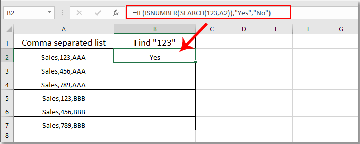
Megjegyzések: A képletben A2 a cella tartalmazza a vesszővel elválasztott értékeket.

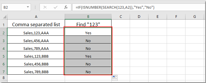
2. Folyamatosan válassza ki az eredmény cellát, és az összes eredmény eléréséhez húzza lefelé a Kitöltő kezelőt. Ha a „123” érték szerepel a vesszővel elválasztott cellákban, akkor az eredmény „Igen”; különben az eredményt nemként kapja meg. Lásd a képernyőképet:


Kapcsolódó cikkek:

A legjobb irodai hatékonyságnövelő eszközök

🤖 Kutools AI Aide: Forradalmasítsa az adatelemzést a következők alapján: Intelligens végrehajtás   |  Kód létrehozása  |  Hozzon létre egyéni képleteket  |  Adatok elemzése és diagramok létrehozása  |  A Kutools funkciók meghívása...
Népszerű szolgáltatások: Ismétlődések keresése, kiemelése vagy azonosítása   |  Üres sorok törlése   |  Oszlopok vagy cellák kombinálása adatvesztés nélkül   |   Kerek Formula nélkül ...
Szuper keresés: Több kritérium VLookup    Többértékű VLookup  |   VLookup több munkalapon   |   Fuzzy Lookup ....
Speciális legördülő lista: Gyors legördülő lista létrehozása   |  Függő legördülő lista   |  Többszörösen válassza ki a legördülő listát ....
Oszlopkezelő: Adjon meg egy adott számú oszlopot  |  Oszlopok mozgatása  |  Kapcsolja be a Rejtett oszlopok láthatósági állapotát  |  Tartományok és oszlopok összehasonlítása ...
Kiemelt funkciók: Rács fókusz   |  Design nézet   |   Nagy Formula bár    Munkafüzet és lapkezelő   |  Erőforrás-könyvtár (Auto szöveg)   |  Dátumválasztó   |  Kombinálja a munkalapokat   |  Cellák titkosítása/dekódolása    E-mailek küldése listánként   |  Szuper szűrő   |   Speciális szűrő (félkövér/dőlt/áthúzott szűrés...) ...
A 15 legjobb eszközkészlet12 szöveg Eszközök (Szöveg hozzáadása, Karakterek eltávolítása,...)   |   50 + Táblázatos Típusai (Gantt-diagram,...)   |   40+ Praktikus képletek (Számolja ki az életkort a születésnap alapján,...)   |   19 beszúrás Eszközök (Helyezze be a QR-kódot, Kép beszúrása az útvonalból,...)   |   12 Átalakítás Eszközök (Számok szavakig, Valuta átváltás,...)   |   7 Egyesítés és felosztás Eszközök (Haladó kombinált sorok, Hasított sejtek,...)   |   ... és több

Töltsd fel Excel-készségeidet a Kutools for Excel segítségével, és tapasztald meg a még soha nem látott hatékonyságot. A Kutools for Excel több mint 300 speciális funkciót kínál a termelékenység fokozásához és az időmegtakarításhoz.  Kattintson ide, hogy megszerezze a leginkább szükséges funkciót...

Leírás


Az Office lap füles felületet hoz az Office-ba, és sokkal könnyebbé teszi a munkáját

  • Füles szerkesztés és olvasás engedélyezése Wordben, Excelben és PowerPointban, Publisher, Access, Visio és Project.
  • Több dokumentum megnyitása és létrehozása ugyanazon ablak új lapjain, mint új ablakokban.
  • 50% -kal növeli a termelékenységet, és naponta több száz kattintással csökkenti az egér kattintását!
Comments (17)
No ratings yet. Be the first to rate!
This comment was minimized by the moderator on the site
It’s working for single value, how do I find multiple values. Example: search values (101, 402,110) it might have all 3 or only one or two values and find cell will have any of three or all three or two.
Scenarios
1. Cell 1: 101 cell 2: 101,402,110,202,220
2. Cell 1: 101,402 cell 2: 101,402,202,220,110
3. Cell 1: 110,101,402 cell 2: 101,402,202,220,110

Pls advice
This comment was minimized by the moderator on the site
Hey, I still cant figure this out. I am still having the same problem. instead of using number in the formula I am using a cell reference. for example if i am searching for "1"(Q$1) in (123, 25,29,200)($J2) it is still giving me YES. The formula is =IF(ISNUMBER(SEARCH(Q$1,$J2)),"yes","no")

PS: I have a big data set I cannot put commas before and after in every cell. Will appreciate a solution
This comment was minimized by the moderator on the site
Hi Hassam

Just use the following formula without the IF function. If the number matches exactly, you will get the result "TRUE", otherwise you will get the result "FALSE".
=ISNUMBER(FIND(",1,",","&$J2&","))
https://www.extendoffice.com/images/stories/comments/comment-picture-zxm/match.png
This comment was minimized by the moderator on the site
Hi All, I have a cell that has multiple countries separated by commas
Example : A2 cell value is (India, Japan, Malaysia, Greater China)
Column G has the country names
Now , I need to find look for a formula that compares value from column G to value in A2 cell .
If the value matches, then return true otherwise return False
This comment was minimized by the moderator on the site
Hi Mohini Verma,
The formula can be modified as follows:
=IF(ISNUMBER(SEARCH(G2,A2)),"TRUE","FALSE")
This comment was minimized by the moderator on the site
How about this please, I need to get the values in A and equate them with the figures in C and return the values in B separated as in commas respectively to C.

Thanks
This comment was minimized by the moderator on the site
Hi duncan,
If you are using Excel for 365, the following formula can help solving the problem.
=TEXTJOIN(",",TRUE,XLOOKUP(TRANSPOSE(VALUE(TEXTSPLIT(D1,","))),A1:A3,B1:B3,"",0,1))
This formula only works in Excel for 365. For other Excel versions other than Excel for 365, I have not found a formula that handles it..
https://www.extendoffice.com/images/stories/comments/comment-picture-zxm/find-value.png
This comment was minimized by the moderator on the site
Hi Please help

I have table in Excel with two columns A & B, under A there are value Eg A2 Cell has 1,2,2,1,2,1,2 etc ( only has two numbers 1 and 2 but needs to recognise it has only 1 & 2 in the whole cell and no other number) and A3 has 1,1,1 and A4 has 0, A5 has 2,2,2,2 and A6 has 20. i want B2 should return the value for A2 as Asia, B3 Africa, B4 as None, B5 as America and B6 as Europe. I thought i could use the if formula but it is not able to recognise comma separated numbers and return value). Please Help
This comment was minimized by the moderator on the site
Hello!
This is a really cool formula, but it has ... flaw? ... that I cannot figure out how to work around it. "Flaw" is not the correct word, but I cannot think (it's 8:30 am on Monday) of the right word.
When you are looking for any part of a number, you get "yes". So, the following all return "yes":
=IF(ISNUMBER(SEARCH(12,A2)),"yes","no")
=IF(ISNUMBER(SEARCH(23,A2)),"yes","no")
=IF(ISNUMBER(SEARCH(3,A2)),"yes","no")

I tried wrapping the numbers in quotes to no avail. The formula works perfectly for the example's use case, in which all of the numbers are of the same length. But if you are looking for a shorter number that happens to appear in the string, you get a false positive.
Is there an alternative to "SEARCH" that is more literal (again, is that the word? haha)? 
Thanks! 
This comment was minimized by the moderator on the site
Hi Scott S.,Do you mean search for the exact string?
This comment was minimized by the moderator on the site
Hi, Crystal.
Yes, I suppose that is the way to phrase it. 
The current solution will return “Yes” for any part of the number string. So the numbers 1, 2, 3, 12, 23, and 123 will all return “Yes”. 
I have been trying to come up with a solution that will search a string of numbers and return “Yes” for an exact match. 
This comment was minimized by the moderator on the site
Hi Scott S,Thanks for your feedback. I haven't found the solution yet and will get back to you if I found it.
This comment was minimized by the moderator on the site
I have found a solution. If you add a comma to the left and right of your list it will require the search function to find an exact match from comma to comma. See example below:
=IF(ISNUMBER(SEARCH(",12,",A2)),"yes","no")

,312,123,10,112,126,
This will return false because there is no variable from comma to comma (,12,) that matches the search. 
If you need further clarification let me know and ill post a better example.I was having the same problem when automating a report for my boss and had an epiphany. :)
This comment was minimized by the moderator on the site
Hey, I still cant figure this out. I am still having the same problem. instead of using number in the formula I am using a cell reference. for example if i am searching for "1"(Q$1) in (123, 25,29,200)($J2) it is still giving me YES. The formula is =IF(ISNUMBER(SEARCH(Q$1,$J2)),"yes","no")

PS: I have a big data set I cannot put commas before and after in every cell. Will appreciate a solution
This comment was minimized by the moderator on the site
I have found a solution for this. If you add a comma to the left and right of your list and include them (like a sandwich) in your search it'll allow you to find an exact match. Example below:
,123,231,321,122,321,1,2,3,23,
SEARCH(",23,")
This way it forces the search to match from one comma to the other rather than just part of the entry from the list. Hope this is what you were looking for?
This comment was minimized by the moderator on the site
Good Morning to all.I have a excel question that how to count comma separated specific values in a single cell in excel.I want to count no of 15's in a single cell that contains 15,215,15,155,45,1515,15 I need the result 3. Is there any formula in excel.
This comment was minimized by the moderator on the site
Yes, there is a function in Excel that can do this for you. However, as explained in the problem above to gain better accuracy for your data add a comma to the left and right of your list and include it in your search. See example below:
,15,215,15,155,45,1515,15,
=COUNTIF(A1, ",15,")
The explanation of this formula is as follows: =COUNTIF(cell number or range, value your looking for/counting)
Let me know if you need a better example.
There are no comments posted here yet
Please leave your comments in English
Posting as Guest
×
Rate this post:
0   Characters
Suggested Locations