Ugrás a tartalomra

Hogyan lehet kiemelni az aktív cellát vagy kiválasztást az Excelben?

Ha nagy munkalapja van, talán nehéz egy pillanat alatt megtudnia az aktív cellát vagy az aktív kijelölést. De ha az aktív cella / szakasz kiemelkedő színű, akkor kideríteni, hogy nem jelent problémát. Ebben a cikkben arról fogok beszélni, hogyan lehet automatikusan kiemelni az aktív cellát vagy a kiválasztott cellatartományt az Excel programban.

Jelölje ki az aktív cellát vagy kijelölést VBA kóddal


nyíl kék jobb buborék Jelölje ki az aktív cellát vagy kijelölést VBA kóddal

A következő VBA-kód segíthet kiemelni az aktív cellát vagy kiválasztást dinamikusan, kérjük, tegye a következőket:

1. Tartsa lenyomva a ALT + F11 billentyűk megnyitásához Microsoft Visual Basic for Applications ablak.

2. Ezután válasszon Ez a munkafüzet balról Project Explorer, kattintson duplán a fájl megnyitásához Modulok, majd másolja és illessze be a következő VBA kódot az üres modulba:

VBA kód: Jelölje ki az aktív cellát vagy kijelölést

Sub Workbook_SheetSelectionChange(ByVal Sh As Object, ByVal Target As Excel.Range)
'Update 20140923
Static xLastRng As Range
On Error Resume Next
Target.Interior.ColorIndex = 6
xLastRng.Interior.ColorIndex = xlColorIndexNone
Set xLastRng = Target
End Sub

doc-kiemelés-aktív-sejt-1

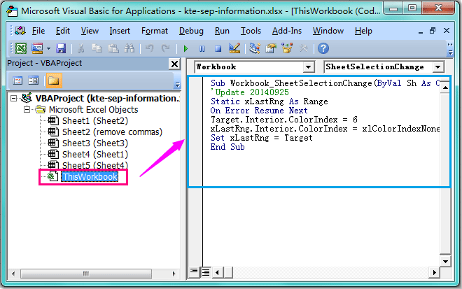
3. Ezután mentse el és zárja be ezt a kódot, és térjen vissza a munkalapra. Most, amikor egy cellát vagy kijelölést választ, a kijelölt cellák kiemelésre kerülnek, és dinamikusan mozognak a kiválasztott cellák változásával.

Megjegyzések:

1. Ha nem találja a Projekt Explorer panel az ablakban kattintson Megnézem > Project Explorer a Microsoft Visual Basic for Applications ablak megnyitni.

2. A fenti kódban megváltoztathatja .ColorIndex = 6 szín más színre tetszik.

3. Ez a VBA kód alkalmazható a munkafüzet összes munkalapjára.

4. Ha van néhány színes cella a munkalapon, akkor a szín elvész, amikor rákattint a cellára, majd átkerül egy másik cellába.


Kapcsolódó cikk:

Hogyan lehet automatikusan kiemelni az Excel aktív cellájának sorát és oszlopát?

A legjobb irodai hatékonyságnövelő eszközök

🤖 Kutools AI Aide: Forradalmasítsa az adatelemzést a következők alapján: Intelligens végrehajtás   |  Kód létrehozása  |  Hozzon létre egyéni képleteket  |  Adatok elemzése és diagramok létrehozása  |  A Kutools funkciók meghívása...
Népszerű szolgáltatások: Ismétlődések keresése, kiemelése vagy azonosítása   |  Üres sorok törlése   |  Oszlopok vagy cellák kombinálása adatvesztés nélkül   |   Kerek Formula nélkül ...
Szuper keresés: Több kritérium VLookup    Többértékű VLookup  |   VLookup több munkalapon   |   Fuzzy Lookup ....
Speciális legördülő lista: Gyors legördülő lista létrehozása   |  Függő legördülő lista   |  Többszörösen válassza ki a legördülő listát ....
Oszlopkezelő: Adjon meg egy adott számú oszlopot  |  Oszlopok mozgatása  |  Kapcsolja be a Rejtett oszlopok láthatósági állapotát  |  Tartományok és oszlopok összehasonlítása ...
Kiemelt funkciók: Rács fókusz   |  Design nézet   |   Nagy Formula bár    Munkafüzet és lapkezelő   |  Erőforrás-könyvtár (Auto szöveg)   |  Dátumválasztó   |  Kombinálja a munkalapokat   |  Cellák titkosítása/dekódolása    E-mailek küldése listánként   |  Szuper szűrő   |   Speciális szűrő (félkövér/dőlt/áthúzott szűrés...) ...
A 15 legjobb eszközkészlet12 szöveg Eszközök (Szöveg hozzáadása, Karakterek eltávolítása,...)   |   50 + Táblázatos Típusai (Gantt-diagram,...)   |   40+ Praktikus képletek (Számolja ki az életkort a születésnap alapján,...)   |   19 beszúrás Eszközök (Helyezze be a QR-kódot, Kép beszúrása az útvonalból,...)   |   12 Átalakítás Eszközök (Számok szavakig, Valuta átváltás,...)   |   7 Egyesítés és felosztás Eszközök (Haladó kombinált sorok, Hasított sejtek,...)   |   ... és több

Töltsd fel Excel-készségeidet a Kutools for Excel segítségével, és tapasztald meg a még soha nem látott hatékonyságot. A Kutools for Excel több mint 300 speciális funkciót kínál a termelékenység fokozásához és az időmegtakarításhoz.  Kattintson ide, hogy megszerezze a leginkább szükséges funkciót...

Leírás


Az Office lap füles felületet hoz az Office-ba, és sokkal könnyebbé teszi a munkáját

  • Füles szerkesztés és olvasás engedélyezése Wordben, Excelben és PowerPointban, Publisher, Access, Visio és Project.
  • Több dokumentum megnyitása és létrehozása ugyanazon ablak új lapjain, mint új ablakokban.
  • 50% -kal növeli a termelékenységet, és naponta több száz kattintással csökkenti az egér kattintását!
Comments (16)
No ratings yet. Be the first to rate!
This comment was minimized by the moderator on the site
I had the same problem, read the whole page and comments. While thinking to apply it or not, I was just randomly clicking on number and letters to select the whole column and rows. Then suddenly highlight of selected cell feature came back :)
This comment was minimized by the moderator on the site
Hello, if someone can help me... I pick up this code in internet (apologies to the owner). It does almost what i need but this code select the entirerow. What i need is a change that alow to select just the first two cells of the row of the activecells. When i click in the cell, i need that the cell of the column "$I16" and "$J16" (16 is the first line of my table) of that row became interior color (=9359529). The code is this: 
Dim lTarget As Range

Private Sub Worksheet_SelectionChange(ByVal Target As Range)

If Target.Row >= 16 Then

If Not lTarget Is Nothing Then

lTarget.EntireRow.Interior.ColorIndex = 0
End If

Target.EntireRow.Interior.Color = 9359529

Set lTarget = Target
End If
End Sub

Can you help me? I had try to change this code but the only thing i can as the select the interior color of the cell target and not the column "$I" and "$J" in that specific row.Thank you for your help.
Luis Lopes
This comment was minimized by the moderator on the site
I know that you proposed a solution but the solution comes with another problem as you described below: "The only problem with having this code active is that you can no longer change the active cell color as it changes back to what it was before you clicked it. I suggest that if you need to change the highlight colors on the sheet, do so with macros disabled or change the sub name for a second so it doesn't trigger when you are clicking on cells". This is not an acceptable alternative for me. I need to be able to change the colors in the cells when the macro is active. Do you have a solution for this this problem. If you come up with a solution for this problem please republish your corrected macro the new macro in full (rather than proposing patches to your original macro because I am technically challenged as far as macro are concerned).
This comment was minimized by the moderator on the site
I tried your macro by copying and pasting it into my Excel file. I did change one thing in the macro though. I changed the color index from 6 to 24 (to a color different than the colors I am currently using in my macro). It worked very nicely and I liked it a lot but then started causing a problem for me. I have a lot of cells filled with with colors in my Excel. The macro started removing the color fill from every cell touched. I don't know how to stop the macro's this odd behavior. I did not have any choice but to remove the macro from my file. I still like to use this macro if someone can help me to fix it.
This comment was minimized by the moderator on the site
That was super helpful, thank you.
This comment was minimized by the moderator on the site
Anyway you can do the left adjacent cell to highlight instead of active cell? Or a range of cells around the activecell?
This comment was minimized by the moderator on the site
Thank you, but use this with caution. It has the undesirable counter effect of not letting undo. Is there any solution for that?
This comment was minimized by the moderator on the site
But i am unable to do undo option and lose the previously assigned cell color also.
Please provide solution
This comment was minimized by the moderator on the site
Perfect solution as I always tend to loose the track of the highlighted cell during "Find and Select" operation. Thanks a lot.
This comment was minimized by the moderator on the site
Great!! But what if I don't want to lose the previously assigned cell color? That would be greater to know.
This comment was minimized by the moderator on the site
Use a conditional format on the cells you want to protect.
This comment was minimized by the moderator on the site
Instead of "ColorIndex" which has a limited set of 255 values (meaning any custom colors are lost), use "Color" instead. You'll need to store the old value in a new static long variable and also generate the highlight color you want with the RGB function. The only problem with having this code active is that you can no longer change the active cell color as it changes back to what it was before you clicked it. I suggest that if you need to change the highlight colors on the sheet, do so with macros disabled or change the sub name for a second so it doesn't trigger when you are clicking on cells, then just rename it back to normal to "re-activate" it. Here is my code:

Sub Workbook_SheetSelectionChange(ByVal Sh As Object, ByVal Target As Excel.Range)

Static xLastRng As Range
Static xLastRngColor As Long

On Error Resume Next

xLastRng.Interior.Color = xLastRngColor
xLastRngColor = Target.Interior.Color
Target.Interior.Color = RGB(255, 255, 0) 'compose whatever highlight color you want with RGB values, I am using yellow here
Set xLastRng = Target

End Sub
This comment was minimized by the moderator on the site
work.... great...
This comment was minimized by the moderator on the site
Yes, I would like to know this as well. How would you keep the previously selected cells highlight for tracking purposes?
This comment was minimized by the moderator on the site
See my comment above.
There are no comments posted here yet
Load More
Please leave your comments in English
Posting as Guest
×
Rate this post:
0   Characters
Suggested Locations